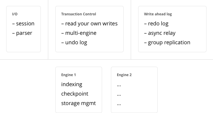
Storing data with vinyl
Tarantool is a transactional and persistent DBMS that maintains 100% of its data in RAM. The greatest advantages of in-memory databases are their speed and ease of use: they demonstrate consistently high performance, but you never need to tune them.
A few years ago we decided to extend the product by implementing a classical storage engine similar to those used by regular DBMSs: it uses RAM for caching, while the bulk of its data is stored on disk. We decided to make it possible to set a storage engine independently for each table in the database, which is the same way that MySQL approaches it, but we also wanted to support transactions from the very beginning.
The first question we needed to answer was whether to create our own storage engine or use an existing library. The open-source community offered a few viable solutions. The RocksDB library was the fastest growing open-source library and is currently one of the most prominent out there. There were also several lesser-known libraries to consider, such as WiredTiger, ForestDB, NestDB, and LMDB.
Nevertheless, after studying the source code of existing libraries and considering the pros and cons, we opted for our own storage engine. One reason is that the existing third-party libraries expected requests to come from multiple operating system threads and thus contained complex synchronization primitives for controlling parallel data access. If we had decided to embed one of these in Tarantool, we would have made our users bear the overhead of a multithreaded application without getting anything in return. The thing is, Tarantool has an actor-based architecture. The way it processes transactions in a dedicated thread allows it to do away with the unnecessary locks, interprocess communication, and other overhead that accounts for up to 80% of processor time in multithreaded DBMSs.
The Tarantool process consists of a fixed number of “actor” threads
If you design a database engine with cooperative multitasking in mind right from the start, it not only significantly speeds up the development process, but also allows the implementation of certain optimization tricks that would be too complex for multithreaded engines. In short, using a third-party solution wouldn’t have yielded the best result.
Once the idea of using an existing library was off the table, we needed to pick an architecture to build upon. There are two competing approaches to on-disk data storage: the older one relies on B-trees and their variations; the newer one advocates the use of log-structured merge-trees, or “LSM” trees. MySQL, PostgreSQL, and Oracle use B-trees, while Cassandra, MongoDB, and CockroachDB have adopted LSM trees.
B-trees are considered better suited for reads and LSM trees—for writes. However, with SSDs becoming more widespread and the fact that SSDs have read throughput that’s several times greater than write throughput, the advantages of LSM trees in most scenarios was more obvious to us.
Before dissecting LSM trees in Tarantool, let’s take a look at how they work. To do that, we’ll begin by analyzing a regular B-tree and the issues it faces. A B-tree is a balanced tree made up of blocks, which contain sorted lists of key- value pairs. (Topics such as filling and balancing a B-tree or splitting and merging blocks are outside of the scope of this article and can easily be found on Wikipedia). As a result, we get a container sorted by key, where the smallest element is stored in the leftmost node and the largest one in the rightmost node. Let’s have a look at how insertions and searches in a B-tree happen.
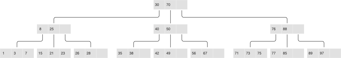
Classical B-tree
If you need to find an element or check its membership, the search starts at the
root, as usual. If the key is found in the root block, the search stops;
otherwise, the search visits the rightmost block holding the largest element
that’s not larger than the key being searched (recall that elements at each
level are sorted). If the first level yields no results, the search proceeds to
the next level. Finally, the search ends up in one of the leaves and probably
locates the needed key. Blocks are stored and read into RAM one by one, meaning
the algorithm reads  blocks in a single search, where N is the number of
elements in the B-tree. In the simplest case, writes are done similarly: the
algorithm finds the block that holds the necessary element and updates (inserts)
its value.
blocks in a single search, where N is the number of
elements in the B-tree. In the simplest case, writes are done similarly: the
algorithm finds the block that holds the necessary element and updates (inserts)
its value.
To better understand the data structure, let’s consider a practical example: say we have a B-tree with 100,000,000 nodes, a block size of 4096 bytes, and an element size of 100 bytes. Thus each block will hold up to 40 elements (all overhead considered), and the B-tree will consist of around 2,570,000 blocks and 5 levels: the first four will have a size of 256 Mb, while the last one will grow up to 10 Gb. Obviously, any modern computer will be able to store all of the levels except the last one in filesystem cache, so read requests will require just a single I/O operation.
But if we change our perspective —B-trees don’t look so good anymore. Suppose we need to update a single element. Since working with B-trees involves reading and writing whole blocks, we would have to read in one whole block, change our 100 bytes out of 4096, and then write the whole updated block to disk. In other words,we were forced to write 40 times more data than we actually modified!
If you take into account the fact that an SSD block has a size of 64 Kb+ and not every modification changes a whole element, the extra disk workload can be greater still.
Authors of specialized literature and blogs dedicated to on-disk data storage have coined two terms for these phenomena: extra reads are referred to as “read amplification” and writes as “write amplification”.
The amplification factor (multiplication coefficient) is calculated as the ratio of the size of actual read (or written) data to the size of data needed (or actually changed). In our B-tree example, the amplification factor would be around 40 for both reads and writes.
The huge number of extra I/O operations associated with updating data is one of the main issues addressed by LSM trees. Let’s see how they work.
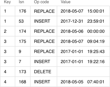
The key difference between LSM trees and regular B-trees is that LSM trees don’t just store data (keys and values), but also data operations: insertions and deletions.

LSM tree:
- Stores statements, not values:
- REPLACE
- DELETE
- UPSERT
- Every statement is marked by LSN
- Append-only files, garbage is collected after a checkpoint
- Transactional log of all filesystem changes: vylog
For example, an element corresponding to an insertion operation has, apart from a key and a value, an extra byte with an operation code (“REPLACE” in the image above). An element representing the deletion operation contains a key (since storing a value is unnecessary) and the corresponding operation code—“DELETE”. Also, each LSM tree element has a log sequence number (LSN), which is the value of a monotonically increasing sequence that uniquely identifies each operation. The whole tree is first ordered by key in ascending order, and then, within a single key scope, by LSN in descending order.
A single level of an LSM tree
Unlike a B-tree, which is stored completely on disk and can be partly cached in RAM, when using an LSM tree, memory is explicitly separated from disk right from the start. The issue of volatile memory and data persistence is beyond the scope of the storage algorithm and can be solved in various ways—for example, by logging changes.
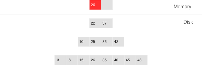
The part of an LSM tree that’s stored in RAM is called L0 (level zero). The size
of RAM is limited, so L0 is allocated a fixed amount of memory. For example, in
Tarantool, the L0 size is controlled by the vinyl_memory parameter. Initially,
when an LSM tree is empty, operations are written to L0. Recall that all
elements are ordered by key in ascending order, and then within a single key
scope, by LSN in descending order, so when a new value associated with a given
key gets inserted, it’s easy to locate the older value and delete it. L0 can be
structured as any container capable of storing a sorted sequence of elements.
For example, in Tarantool, L0 is implemented as a B+*-tree. Lookups and
insertions are standard operations for the data structure underlying L0, so I
won’t dwell on those.
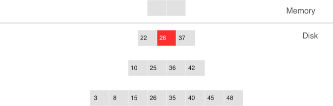
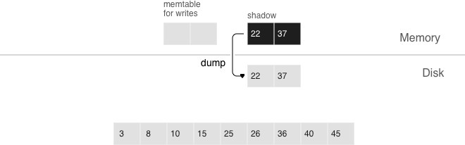
Sooner or later the number of elements in an LSM tree exceeds the L0 size and that’s when L0 gets written to a file on disk (called a “run”) and then cleared for storing new elements. This operation is called a “dump”.
Dumps on disk form a sequence ordered by LSN: LSN ranges in different runs don’t overlap, and the leftmost runs (at the head of the sequence) hold newer operations. Think of these runs as a pyramid, with the newest ones closer to the top. As runs keep getting dumped, the pyramid grows higher. Note that newer runs may contain deletions or replacements for existing keys. To remove older data, it’s necessary to perform garbage collection (this process is sometimes called “merge” or “compaction”) by combining several older runs into a new one. If two versions of the same key are encountered during a compaction, only the newer one is retained; however, if a key insertion is followed by a deletion, then both operations can be discarded.
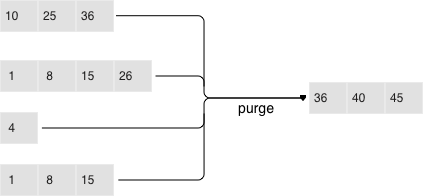
The key choices determining an LSM tree’s efficiency are which runs to compact and when to compact them. Suppose an LSM tree stores a monotonically increasing sequence of keys (1, 2, 3, …,) with no deletions. In this case, compacting runs would be useless: all of the elements are sorted, the tree doesn’t have any garbage, and the location of any key can unequivocally be determined. On the other hand, if an LSM tree contains many deletions, doing a compaction would free up some disk space. However, even if there are no deletions, but key ranges in different runs overlap a lot, compacting such runs could speed up lookups as there would be fewer runs to scan. In this case, it might make sense to compact runs after each dump. But keep in mind that a compaction causes all data stored on disk to be overwritten, so with few reads it’s recommended to perform it less often.
To ensure it’s optimally configurable for any of the scenarios above, an LSM tree organizes all runs into a pyramid: the newer the data operations, the higher up the pyramid they are located. During a compaction, the algorithm picks two or more neighboring runs of approximately equal size, if possible.
- Multi-level compaction can span any number of levels
- A level can contain multiple runs
All of the neighboring runs of approximately equal size constitute an LSM tree level on disk. The ratio of run sizes at different levels determines the pyramid’s proportions, which allows optimizing the tree for write-intensive or read-intensive scenarios.
Suppose the L0 size is 100 Mb, the ratio of run sizes at each level (the
vinyl_run_size_ratio parameter) is 5, and there can be no more than 2 runs per
level (the vinyl_run_count_per_level parameter). After the first 3 dumps, the
disk will contain 3 runs of 100 Mb each—which constitute L1 (level one). Since 3
> 2, the runs will be compacted into a single 300 Mb run, with the older ones
being deleted. After 2 more dumps, there will be another compaction, this time
of 2 runs of 100 Mb each and the 300 Mb run, which will produce one 500 Mb run.
It will be moved to L2 (recall that the run size ratio is 5), leaving L1 empty.
The next 10 dumps will result in L2 having 3 runs of 500 Mb each, which will be
compacted into a single 1500 Mb run. Over the course of 10 more dumps, the
following will happen: 3 runs of 100 Mb each will be compacted twice, as will
two 100 Mb runs and one 300 Mb run, which will yield 2 new 500 Mb runs in L2.
Since L2 now has 3 runs, they will also be compacted: two 500 Mb runs and one
1500 Mb run will produce a 2500 Mb run that will be moved to L3, given its size.
This can go on infinitely, but if an LSM tree contains lots of deletions, the resulting compacted run can be moved not only down, but also up the pyramid due to its size being smaller than the sizes of the original runs that were compacted. In other words, it’s enough to logically track which level a certain run belongs to, based on the run size and the smallest and greatest LSN among all of its operations.
If it’s necessary to reduce the number of runs for lookups, then the run size
ratio can be increased, thus bringing the number of levels down. If, on the
other hand, you need to minimize the compaction-related overhead, then the run
size ratio can be decreased: the pyramid will grow higher, and even though runs
will be compacted more often, they will be smaller, which will reduce the total
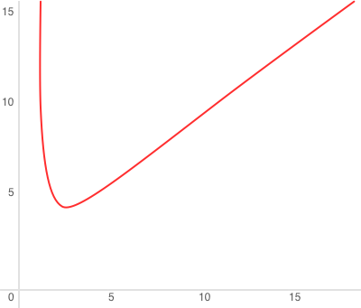
amount of work done. In general, write amplification in an LSM tree is described
by this formula:  or, alternatively,
 , where N is
the total size of all tree elements, L0 is the level zero size, and x is the
level size ratio (the
, where N is
the total size of all tree elements, L0 is the level zero size, and x is the
level size ratio (the level_size_ratio parameter). At  = 40 (the disk-to-
memory ratio), the plot would look something like this:
= 40 (the disk-to-
memory ratio), the plot would look something like this:
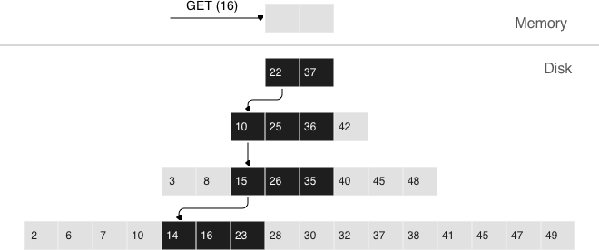
As for read amplification, it’s proportional to the number of levels. The lookup
cost at each level is no greater than that for a B-tree. Getting back to the
example of a tree with 100,000,000 elements: given 256 Mb of RAM and the default
values of vinyl_run_size_ratio and vinyl_run_count_per_level, write
amplification would come out to about 13, while read amplification could be as
high as 150. Let’s try to figure out why this happens.
When doing a lookup in an LSM tree, what we need to find is not the element itself, but the most recent operation associated with it. If it’s a deletion, then the tree doesn’t contain this element. If it’s an insertion, we need to grab the topmost value in the pyramid, and the search can be stopped after finding the first matching key. In the worst-case scenario, that is if the tree doesn’t hold the needed element, the algorithm will have to sequentially visit all of the levels, starting from L0.
Unfortunately, this scenario is quite common in real life. For example, when inserting a value into a tree, it’s necessary to make sure there are no duplicates among primary/unique keys. So to speed up membership checks, LSM trees use a probabilistic data structure called a “Bloom filter”, which will be covered a bit later, in a section on how vinyl works under the hood.
In the case of a single-key search, the algorithm stops after encountering the first match. However, when searching within a certain key range (for example, looking for all the users with the last name “Ivanov”), it’s necessary to scan all tree levels.

Searching within a range of [24,30)
The required range is formed the same way as when compacting several runs: the algorithm picks the key with the largest LSN out of all the sources, ignoring the other associated operations, then moves on to the next key and repeats the procedure.
Why would one store deletions? And why doesn’t it lead to a tree overflow in the case of for i=1,10000000 put(i) delete(i) end?
With regards to lookups, deletions signal the absence of a value being searched; with compactions, they clear the tree of “garbage” records with older LSNs.
While the data is in RAM only, there’s no need to store deletions. Similarly, you don’t need to keep them following a compaction if they affect, among other things, the lowest tree level, which contains the oldest dump. Indeed, if a value can’t be found at the lowest level, then it doesn’t exist in the tree.
- We can’t delete from append-only files
- Tombstones (delete markers) are inserted into L0 instead
Deletion, step 1: a tombstone is inserted into L0
Deletion, step 2: the tombstone passes through intermediate levels

Deletion, step 3: in the case of a major compaction, the tombstone is removed from the tree
If a deletion is known to come right after the insertion of a unique value, which is often the case when modifying a value in a secondary index, then the deletion can safely be filtered out while compacting intermediate tree levels. This optimization is implemented in vinyl.
Apart from decreasing write amplification, the approach that involves periodically dumping level L0 and compacting levels L1-Lk has a few advantages over the approach to writes adopted by B-trees:
- Dumps and compactions write relatively large files: typically, the L0 size is 50-100 Mb, which is thousands of times larger than the size of a B-tree block.
- This large size allows efficiently compressing data before writing it. Tarantool compresses data automatically, which further decreases write amplification.
- There is no fragmentation overhead, since there’s no padding/empty space between the elements inside a run.
- All operations create new runs instead of modifying older data in place. This allows avoiding those nasty locks that everyone hates so much. Several operations can run in parallel without causing any conflicts. This also simplifies making backups and moving data to replicas.
- Storing older versions of data allows for the efficient implementation of transaction support by using multiversion concurrency control.
One of the key advantages of the B-tree as a search data structure is its
predictability: all operations take no longer than  to run.
Conversely, in a classical LSM tree, both read and write speeds can differ by a
factor of hundreds (best case scenario) or even thousands (worst case scenario).
For example, adding just one element to L0 can cause it to overflow, which can
trigger a chain reaction in levels L1, L2, and so on. Lookups may find the
needed element in L0 or may need to scan all of the tree levels. It’s also
necessary to optimize reads within a single level to achieve speeds comparable
to those of a B-tree. Fortunately, most disadvantages can be mitigated or even
eliminated with additional algorithms and data structures. Let’s take a closer
look at these disadvantages and how they’re dealt with in Tarantool.
to run.
Conversely, in a classical LSM tree, both read and write speeds can differ by a
factor of hundreds (best case scenario) or even thousands (worst case scenario).
For example, adding just one element to L0 can cause it to overflow, which can
trigger a chain reaction in levels L1, L2, and so on. Lookups may find the
needed element in L0 or may need to scan all of the tree levels. It’s also
necessary to optimize reads within a single level to achieve speeds comparable
to those of a B-tree. Fortunately, most disadvantages can be mitigated or even
eliminated with additional algorithms and data structures. Let’s take a closer
look at these disadvantages and how they’re dealt with in Tarantool.
In an LSM tree, insertions almost always affect L0 only. How do you avoid idle time when the memory area allocated for L0 is full?
Clearing L0 involves two lengthy operations: writing to disk and memory deallocation. To avoid idle time while L0 is being dumped, Tarantool uses writeaheads. Suppose the L0 size is 256 Mb. The disk write speed is 10 Mbps. Then it would take 26 seconds to dump L0. The insertion speed is 10,000 RPS, with each key having a size of 100 bytes. While L0 is being dumped, it’s necessary to reserve 26 Mb of RAM, effectively slicing the L0 size down to 230 Mb.
Tarantool does all of these calculations automatically, constantly updating the
rolling average of the DBMS workload and the histogram of the disk speed. This
allows using L0 as efficiently as possible and it prevents write requests from
timing out. But in the case of workload surges, some wait time is still
possible. That’s why we also introduced an insertion timeout (the
vinyl_timeout parameter), which is set to 60 seconds by default. The write
operation itself is executed in dedicated threads. The number of these threads
(4 by default) is controlled by the vinyl_write_threads parameter. The default
value of 2 allows doing dumps and compactions in parallel, which is also
necessary for ensuring system predictability.
In Tarantool, compactions are always performed independently of dumps, in a separate execution thread. This is made possible by the append-only nature of an LSM tree: after dumps runs are never changed, and compactions simply create new runs.
Delays can also be caused by L0 rotation and the deallocation of memory dumped to disk: during a dump, L0 memory is owned by two operating system threads, a transaction processing thread and a write thread. Even though no elements are being added to the rotated L0, it can still be used for lookups. To avoid read locks when doing lookups, the write thread doesn’t deallocate the dumped memory, instead delegating this task to the transaction processor thread. Following a dump, memory deallocation itself happens instantaneously: to achieve this, L0 uses a special allocator that deallocates all of the memory with a single operation.
- anticipatory dump
- throttling
The dump is performed from the so-called “shadow” L0 without blocking new insertions and lookups
Optimizing reads is the most difficult optimization task with regards to LSM trees. The main complexity factor here is the number of levels: any optimization causes not only much slower lookups, but also tends to require significantly larger RAM resources. Fortunately, the append-only nature of LSM trees allows us to address these problems in ways that would be nontrivial for traditional data structures.
- page index
- bloom filters
- tuple range cache
- multi-level compaction
In B-trees, data compression is either the hardest problem to crack or a great marketing tool—rather than something really useful. In LSM trees, compression works as follows:
During a dump or compaction all of the data within a single run is split into
pages. The page size (in bytes) is controlled by the vinyl_page_size
parameter and can be set separately for each index. A page doesn’t have to be
exactly of vinyl_page_size size—depending on the data it holds, it can be a
little bit smaller or larger. Because of this, pages never have any empty space
inside.
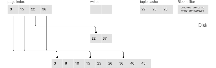
Data is compressed by Facebook’s streaming algorithm called “zstd”. The first key of each page, along with the page offset, is added to a “page index”, which is a separate file that allows the quick retrieval of any page. After a dump or compaction, the page index of the created run is also written to disk.
All .index files are cached in RAM, which allows finding the necessary page
with a single lookup in a .run file (in vinyl, this is the extension of files
resulting from a dump or compaction). Since data within a page is sorted, after
it’s read and decompressed, the needed key can be found using a regular binary
search. Decompression and reads are handled by separate threads, and are
controlled by the vinyl_read_threads parameter.
Tarantool uses a universal file format: for example, the format of a .run file
is no different from that of an .xlog file (log file). This simplifies backup
and recovery as well as the usage of external tools.
Even though using a page index enables scanning fewer pages per run when doing a lookup, it’s still necessary to traverse all of the tree levels. There’s a special case, which involves checking if particular data is absent when scanning all of the tree levels and it’s unavoidable: I’m talking about insertions into a unique index. If the data being inserted already exists, then inserting the same data into a unique index should lead to an error. The only way to throw an error in an LSM tree before a transaction is committed is to do a search before inserting the data. Such reads form a class of their own in the DBMS world and are called “hidden” or “parasitic” reads.
Another operation leading to hidden reads is updating a value in a field on which a secondary index is defined. Secondary keys are regular LSM trees that store differently ordered data. In most cases, in order not to have to store all of the data in all of the indexes, a value associated with a given key is kept in whole only in the primary index (any index that stores both a key and a value is called “covering” or “clustered”), whereas the secondary index only stores the fields on which a secondary index is defined, and the values of the fields that are part of the primary index. Thus, each time a change is made to a value in a field on which a secondary index is defined, it’s necessary to first remove the old key from the secondary index—and only then can the new key be inserted. At update time, the old value is unknown, and it is this value that needs to be read in from the primary key “under the hood”.
For example:
update t1 set city=’Moscow’ where id=1
To minimize the number of disk reads, especially for nonexistent data, nearly all LSM trees use probabilistic data structures, and Tarantool is no exception. A classical Bloom filter is made up of several (usually 3-to-5) bit arrays. When data is written, several hash functions are calculated for each key in order to get corresponding array positions. The bits at these positions are then set to 1. Due to possible hash collisions, some bits might be set to 1 twice. We’re most interested in the bits that remain 0 after all keys have been added. When looking for an element within a run, the same hash functions are applied to produce bit positions in the arrays. If any of the bits at these positions is 0, then the element is definitely not in the run. The probability of a false positive in a Bloom filter is calculated using Bayes’ theorem: each hash function is an independent random variable, so the probability of a collision simultaneously occurring in all of the bit arrays is infinitesimal.
The key advantage of Bloom filters in Tarantool is that they’re easily
configurable. The only parameter that can be specified separately for each index
is called vinyl_bloom_fpr (FPR stands for “false positive ratio”) and it has the
default value of 0.05, which translates to a 5% FPR. Based on this parameter,
Tarantool automatically creates Bloom filters of the optimal size for partial-
key and full-key searches. The Bloom filters are stored in the .index file,
along with the page index, and are cached in RAM.
A lot of people think that caching is a silver bullet that can help with any
performance issue. “When in doubt, add more cache”. In vinyl, caching is viewed
rather as a means of reducing the overall workload and consequently, of getting
a more stable response time for those requests that don’t hit the cache. vinyl
boasts a unique type of cache among transactional systems called a “range tuple
cache”. Unlike, say, RocksDB or MySQL, this cache doesn’t store pages, but
rather ranges of index values obtained from disk, after having performed a
compaction spanning all tree levels. This allows the use of caching for both
single-key and key-range searches. Since this method of caching stores only hot
data and not, say, pages (you may need only some data from a page), RAM is used
in the most efficient way possible. The cache size is controlled by the
vinyl_cache parameter.
Chances are that by now you’ve started losing focus and need a well-deserved dopamine reward. Feel free to take a break, since working through the rest of the article is going to take some serious mental effort.
An LSM tree in vinyl is just a small piece of the puzzle. Even with a single table (or so-called “space”), vinyl creates and maintains several LSM trees, one for each index. But even a single index can be comprised of dozens of LSM trees. Let’s try to understand why this might be necessary.
Recall our example with a tree containing 100,000,000 records, 100 bytes each. As time passes, the lowest LSM level may end up holding a 10 Gb run. During compaction, a temporary run of approximately the same size will be created. Data at intermediate levels takes up some space as well, since the tree may store several operations associated with a single key. In total, storing 10 Gb of actual data may require up to 30 Gb of free space: 10 Gb for the last tree level, 10 Gb for a temporary run, and 10 Gb for the remaining data. But what if the data size is not 10 Gb, but 1 Tb? Requiring that the available disk space always be several times greater than the actual data size is financially unpractical, not to mention that it may take dozens of hours to create a 1 Tb run. And in the case of an emergency shutdown or system restart, the process would have to be started from scratch.
Here’s another scenario. Suppose the primary key is a monotonically increasing sequence—for example, a time series. In this case, most insertions will fall into the right part of the key range, so it wouldn’t make much sense to do a compaction just to append a few million more records to an already huge run.
But what if writes predominantly occur in a particular region of the key range, whereas most reads take place in a different region? How do you optimize the form of the LSM tree in this case? If it’s too high, read performance is impacted; if it’s too low—write speed is reduced.
Tarantool “factorizes” this problem by creating multiple LSM trees for each index. The approximate size of each subtree may be controlled by the vinyl_range_size configuration parameter. We call such subtrees “ranges”.
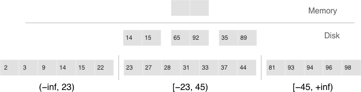
Factorizing large LSM trees via ranging
- Ranges reflect a static layout of sorted runs
- Slices connect a sorted run into a range
Initially, when the index has few elements, it consists of a single range. As more elements are added, its total size may exceed the maximum range size. In that case a special operation called “split” divides the tree into two equal parts. The tree is split at the middle element in the range of keys stored in the tree. For example, if the tree initially stores the full range of -inf…+inf, then after splitting it at the middle key X, we get two subtrees: one that stores the range of -inf…X, and the other storing the range of X…+inf. With this approach, we always know which subtree to use for writes and which one for reads. If the tree contained deletions and each of the neighboring ranges grew smaller as a result, the opposite operation called “coalesce” combines two neighboring trees into one.
Split and coalesce don’t entail a compaction, the creation of new runs, or other
resource-intensive operations. An LSM tree is just a collection of runs. vinyl
has a special metadata log that helps keep track of which run belongs to which
subtree(s). This has the .vylog extension and its format is compatible with an
.xlog file. Similarly to an .xlog file, the metadata log gets rotated at each
checkpoint. To avoid the creation of extra runs with split and coalesce, we have
also introduced an auxiliary entity called “slice”. It’s a reference to a run
containing a key range and it’s stored only in the metadata log. Once the
reference counter drops to zero, the corresponding file gets removed. When it’s
necessary to perform a split or to coalesce, Tarantool creates slice objects for
each new tree, removes older slices, and writes these operations to the metadata
log, which literally stores records that look like this: <tree id, slice id>
or <slice id, run id, min, max>.
This way all of the heavy lifting associated with splitting a tree into two subtrees is postponed until a compaction and then is performed automatically. A huge advantage of dividing all of the keys into ranges is the ability to independently control the L0 size as well as the dump and compaction processes for each subtree, which makes these processes manageable and predictable. Having a separate metadata log also simplifies the implementation of both “truncate” and “drop”. In vinyl, they’re processed instantly, since they only work with the metadata log, while garbage collection is done in the background.
In the previous sections, we mentioned only two operations stored by an LSM tree: deletion and replacement. Let’s take a look at how all of the other operations can be represented. An insertion can be represented via a replacement—you just need to make sure there are no other elements with the specified key. To perform an update, it’s necessary to read the older value from the tree, so it’s easier to represent this operation as a replacement as well—this speeds up future read requests by the key. Besides, an update must return the new value, so there’s no avoiding hidden reads.
In B-trees, the cost of hidden reads is negligible: to update a block, it first needs to be read from disk anyway. Creating a special update operation for an LSM tree that doesn’t cause any hidden reads is really tempting.
Such an operation must contain not only a default value to be inserted if a key has no value yet, but also a list of update operations to perform if a value does exist.
At transaction execution time, Tarantool just saves the operation in an LSM tree, then “executes” it later, during a compaction.
The upsert operation:
space:upsert(tuple, {{operator, field, value}, ... })
- Non-reading update or insert
- Delayed execution
- Background upsert squashing prevents upserts from piling up
Unfortunately, postponing the operation execution until a compaction doesn’t leave much leeway in terms of error handling. That’s why Tarantool tries to validate upserts as fully as possible before writing them to an LSM tree. However, some checks are only possible with older data on hand, for example when the update operation is trying to add a number to a string or to remove a field that doesn’t exist.
A semantically similar operation exists in many products including PostgreSQL and MongoDB. But anywhere you look, it’s just syntactic sugar that combines the update and replace operations without avoiding hidden reads. Most probably, the reason is that LSM trees as data storage structures are relatively new.
Even though an upsert is a very important optimization and implementing it cost us a lot of blood, sweat, and tears, we must admit that it has limited applicability. If a table contains secondary keys or triggers, hidden reads can’t be avoided. But if you have a scenario where secondary keys are not required and the update following the transaction completion will certainly not cause any errors, then the operation is for you.
I’d like to tell you a short story about an upsert. It takes place back when vinyl was only beginning to “mature” and we were using an upsert in production for the first time. We had what seemed like an ideal environment for it: we had tons of keys, the current time was being used as values; update operations were inserting keys or modifying the current time; and we had few reads. Load tests yielded great results.
Nevertheless, after a couple of days, the Tarantool process started eating up 100% of our CPU, and the system performance dropped close to zero.
We started digging into the issue and found out that the distribution of requests across keys was significantly different from what we had seen in the test environment. It was…well, quite nonuniform. Most keys were updated once or twice a day, so the database was idle for the most part, but there were much hotter keys with tens of thousands of updates per day. Tarantool handled those just fine. But in the case of lookups by key with tens of thousands of upserts, things quickly went downhill. To return the most recent value, Tarantool had to read and “replay” the whole history consisting of all of the upserts. When designing upserts, we had hoped this would happen automatically during a compaction, but the process never even got to that stage: the L0 size was more than enough, so there were no dumps.
We solved the problem by adding a background process that performed readaheads on any keys that had more than a few dozen upserts piled up, so all those upserts were squashed and substituted with the read value.
Update is not the only operation where optimizing hidden reads is critical. Even the replace operation, given secondary keys, has to read the older value: it needs to be independently deleted from the secondary indexes, and inserting a new element might not do this, leaving some garbage behind.

If secondary indexes are not unique, then collecting “garbage” from them can be put off until a compaction, which is what we do in Tarantool. The append-only nature of LSM trees allowed us to implement full-blown serializable transactions in vinyl. Read-only requests use older versions of data without blocking any writes. The transaction manager itself is fairly simple for now: in classical terms, it implements the MVTO (multiversion timestamp ordering) class, whereby the winning transaction is the one that finished earlier. There are no locks and associated deadlocks. Strange as it may seem, this is a drawback rather than an advantage: with parallel execution, you can increase the number of successful transactions by simply holding some of them on lock when necessary. We’re planning to improve the transaction manager soon. In the current release, we focused on making the algorithm behave 100% correctly and predictably. For example, our transaction manager is one of the few on the NoSQL market that supports so-called “gap locks”.